Integrating ST and scRNA-seq Data

In this tutorial, we show how to apply CellMirror to integrate ST and scRNA-seq data. As an example, we use the ST data and paired scRNA-seq data of pancreatic ductal adenocarcinoma (PDAC) patient from Moncada , et al. 2020., including 428 spots and 1,926 cells.

Step0: Loading packages (Python)

import warnings
warnings.filterwarnings("ignore")

import os
os.environ['R_HOME'] = '/sibcb2/chenluonanlab7/zuochunman/anaconda3/envs/r4.0/lib/R'
os.environ['R_USER'] = '/sibcb2/chenluonanlab7/zuochunman/anaconda3/envs/CellMirror/lib/python3.8/site-packages/rpy2'

import random
import numpy as np
import scanpy as sc
import matplotlib.pyplot as plt

from CellMirror_utils.utilities import *
from CellMirror_utils.layers import *
from CellMirror_utils.cLDVAE_torch import *
import torch.utils.data as data_utils

parser = parameter_setting()
args = parser.parse_known_args()[0]

# Set seed
np.random.seed(args.seed)
random.seed(args.seed)
torch.manual_seed(args.seed)
torch.cuda.manual_seed(args.seed)

args.lr_cLDVAE = 1e-5; args.gamma = -100

# Set workpath
Save_path = '/sibcb2/chenluonanlab7/zuochunman/Share_data/xiajunjie/PDAC/'

Step1: Reading and preprocessing data (Python)

# Normalization
PDAC_A_st = sc.read_h5ad(Save_path + 'PDAC_A_st.h5ad')
PDAC_A_st.obs['type'] = 'Spatial'
PDAC_A_st.obs['y'] = 100 - PDAC_A_st.obs['y']
PDAC_A_st.obsm['spatial'] = PDAC_A_st.obs[['x','y']].values
sc.pp.normalize_total(PDAC_A_st)
sc.pp.log1p(PDAC_A_st)
sc.pp.highly_variable_genes(PDAC_A_st, flavor='seurat', n_top_genes=3000)

PDAC_A_sc = sc.read_h5ad(Save_path + 'PDAC_A_sc.h5ad')
PDAC_A_sc.obs['type'] = 'SingleCell'
sc.pp.normalize_total(PDAC_A_sc)
sc.pp.log1p(PDAC_A_sc)
sc.pp.highly_variable_genes(PDAC_A_sc, flavor='seurat', n_top_genes=3000)

common_HVGs=np.intersect1d(list(PDAC_A_sc.var.index[PDAC_A_sc.var['highly_variable']]),list(PDAC_A_st.var.index[PDAC_A_st.var['highly_variable']])).tolist()
print(len(common_HVGs))

PDAC_A_st, PDAC_A_sc = PDAC_A_st[:,common_HVGs], PDAC_A_sc[:,common_HVGs]

print('\nShape of target object: ', PDAC_A_st.shape, '\tShape of background object: ', PDAC_A_sc.shape)

# Last batch setting
args = set_last_batchsize(args, PDAC_A_st, PDAC_A_sc)

# Pseudo-data padding
pseudo_st, pseudo_sc = pseudo_data_padding(PDAC_A_st, PDAC_A_sc)

Step2: Training cLDVAE model (Python)

# Dataloader preparation
train = data_utils.TensorDataset(torch.from_numpy(pseudo_st),torch.from_numpy(pseudo_sc))
train_loader = data_utils.DataLoader(train, batch_size=args.batch_size, shuffle=True)

total = data_utils.TensorDataset(torch.from_numpy(pseudo_st),torch.from_numpy(pseudo_sc))
total_loader = data_utils.DataLoader(total, batch_size=args.batch_size, shuffle=False)

# Run cLDVAE
model_cLDVAE = cLDVAE(args=args, n_input=PDAC_A_st.shape[1]).cuda()
history = model_cLDVAE.fit(train_loader, total_loader)

Step3: Saving cLDVAE outputs (Python)

# Pseudo-data deparsing
outputs = model_cLDVAE.predict(total_loader)
PDAC_A_st.obsm['cLDVAE'], PDAC_A_sc.obsm['cLDVAE'] = pseudo_data_deparser(PDAC_A_st, outputs['tg_z_outputs'], PDAC_A_sc, outputs['bg_z_outputs'])

Step4: Implementing MNN on the processed data (Python)

# Run MNN
PDAC_A_st.obsm['CellMirror'], PDAC_A_sc.obsm['CellMirror'] = mnn_correct(PDAC_A_st.obsm['cLDVAE'], PDAC_A_sc.obsm['cLDVAE'])

# Cell type estimation
PDAC_A_st, PDAC_A_sc = estimate_cell_type(PDAC_A_st, PDAC_A_sc, used_obsm='CellMirror', used_label='cell_type_ductal', neighbors=50)

Step5: Saving results for further visualization (Python)

# Save data
colors = np.unique(PDAC_A_sc.obs['cell_type_ductal'].values).tolist()
sc.pl.spatial(PDAC_A_st, img_key=None, color=colors, color_map=plt.cm.get_cmap('plasma'), ncols=5, spot_size=1, frameon=False, show=False)
plt.savefig(Save_path + 'PDAC_A_CellMirror_celltype_proportion.jpg', dpi=100)

PDAC_A_st.obs.to_csv(Save_path + 'PDAC_st_CellMirror_celltype_proportion.csv')
PDAC_A_st.write(Save_path + 'PDAC_A_CellMirror.h5ad', compression='gzip')

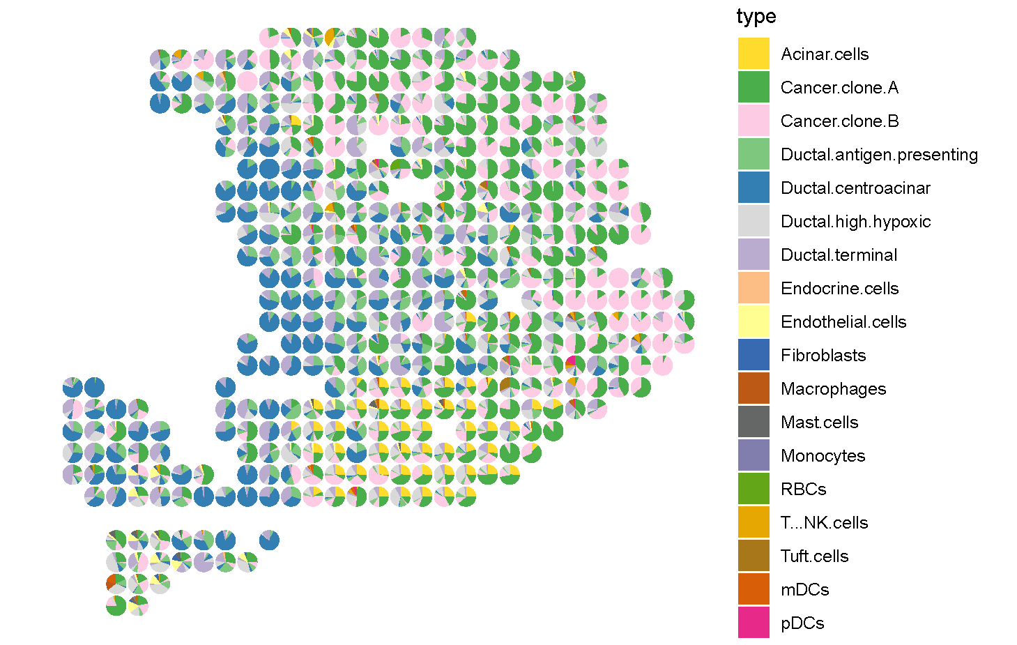
Step6: Visualization (R)

PDAC_st <- read.csv('C:\\Users\\我的电脑\\Desktop\\待办\\PDAC_st_CellMirror_celltype_proportion.csv')
celltypes <- colnames(PDAC_st)[11:dim(PDAC_st)[2]]

suppressMessages(
ggplot2::ggplot()
+ scatterpie::geom_scatterpie(data = PDAC_st, ggplot2::aes(x = x,y = y), cols = celltypes, color = NA,alpha = 1, pie_scale = 0.8)
+ ggplot2::scale_y_reverse()
+ ggplot2::theme_void()
+ ggplot2::coord_fixed(ratio = 1,xlim = NULL, ylim = NULL, expand = TRUE, clip = "on")
+ ggplot2::scale_fill_manual(values = c('Acinar.cells'='#FEDB2C',
                                        'Cancer.clone.A'='#4AAE4B',
                                        'Cancer.clone.B'='#FDCBE4',
                                        'Ductal.antigen.presenting'='#7DC87E',
                                        'Ductal.centroacinar'='#337FB4',
                                        'Ductal.high.hypoxic'='#D9D9D9',
                                        'Ductal.terminal'='#BAACCF',
                                        'Endocrine.cells'='#FCBE84',
                                        'Endothelial.cells'='#FFFF91',
                                        'Fibroblasts'='#386AB2',
                                        'Macrophages'='#BC5914',
                                        'Mast.cells'='#656666',
                                        'Monocytes'='#817EAE',
                                        'RBCs'='#63A618',
                                        'T...NK.cells'='#E7A703',
                                        'Tuft.cells'='#A8771A',
                                        'mDCs'='#D95E08',
                                        'pDCs'='#E72989')))